Writing Your Own Fitting Function
When Should You Do It?
Even though Eddington offers many default fitting functions, sometimes you may want to customize your own fitting function.
Consider the following case: You conduct an experiment to demonstrate the Thin Lens Equation:

After rearranging the equation you get:

You have data records of  and
and  and you want to estimate
  .
You can use our hyperbolic fitting function, but in order to find
You’ll have to do some more calculations with respect to the errors of
the parameters you’ve found.
.
You can use our hyperbolic fitting function, but in order to find
You’ll have to do some more calculations with respect to the errors of
the parameters you’ve found.
A somewhat easier approach would be to use the following fitting function:
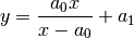
Now, after you fit the data, you get directly (which equals to  )
)
Since this fitting function is not implemented by default, you’d have to implement it yourself.
Basic implementation
A basic implementation of the fitting function presented in the example above would look like this:
from eddington import fitting_function

@fitting_function(n=2)
def lens(a, x):
    return (a[0] * x) / (x - a[0]) + a[1]
We wrap the lens fitting function with the fitting_function decorator
in order to indicate that this function is actually a fitting function. the n
variable indicates how many parameters the fitting function expects. In our example,
we expect 2 parameters: a[0] which is , and a[1] which
encapsulates the systematic errors in our samples.
Note
The inputs of the fitting function are a which is the parameters vector
and x which is the free variable. While a can be from any
array-like type such as list, tuple, numpy.ndarray,
etc. x can be both a numpy.ndarray and float.
Now, we can use the fitting function we’ve created in order to fit the data:
from eddington import FittingData, fit

fitting_data = FittingData.read_from_csv("/path/to/data.csv")  # Load data from file.
fitting_result = fit(fitting_data, lens)  # Do the actual fitting
print(fitting_result)  # Print the results
This usage is more than enough for most use-cases.
Derivatives
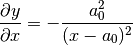
Sometimes, you wish to get an accurate fit, and fast. One way to achieve that is to add derivatives to the fitting function. In our example, we have the following derivatives:
 derivative -
derivative -
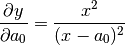
 derivative -

In order to add those derivatives to the fitting function, we should add the
x_derivative and a_derivative to the fitting_function
decorator. In our example:
import numpy as np
from eddington import fitting_function, FittingData, fit


@fitting_function(
    n=2,
    x_derivative=lambda a, x: -np.power(a[0], 2) / np.power(x - a[0], 2),
    a_derivative=lambda a, x: np.stack(
        [
            np.power(x, 2) / np.power(x - a[0], 2),
            np.ones(shape=np.shape(x)),
        ]
    ),
)
def lens(a, x):
    return (a[0] * x) / (x - a[0]) + a[1]
Note
When implementing the derivatives pay attention that you take a as the
first parameter and x as the second. Moreover, make sure that the
dimension of the output x_derivative returns a numpy.ndarray
with dimension similar to x, while a_derivative returns a
numpy.ndarray with dimension equal to x dimension times
a dimension.
The Fitting Functions Registry
By default, creating a new fitting function adds it automatically to the FittingFunctionsRegistry, a singleton containing all fitting functions. Once the fitting function you’ve created is imported (for example, in the __init__.py file) it can be loaded from the registry in the following way:
from eddington import FittingFunctionsRegistry

fit_func = FittingFunctionsRegistry.load("lens")
If you wish to specify a different name to the fitting function by which it can be loaded from the registry, use the name parameter in the fitting_function decorator in the following way:
from eddington import fitting_function, FittingFunctionsRegistry

@fitting_function(n=2, name="my_amazing_func")
def lens(a, x):
    return (a[0] * x) / (x - a[0]) + a[1]

fit_func = FittingFunctionsRegistry.load("my_amazing_func")  # Returns the "lens" function
If you expect others to use your new fitting function, consider adding a syntax string indicating how the fitting functions fit the data. This can be printed out when needed. For example:
from eddington import fitting_function, FittingFunctionsRegistry

@fitting_function(n=2, syntax="(a[0] * x) / (x - a[0]) + a[1]")
def lens(a, x):
    return (a[0] * x) / (x - a[0]) + a[1]

...

fit_func = FittingFunctionsRegistry.load("lens")
print(f"Syntax is: {fit_func.syntax}")  # Prints out the defined syntax
Lastly, if you wish the fitting function to not be saved into the registry, specify
save=False in the fitting_function decorator. For example:
from eddington import fitting_function

@fitting_function(n=2, save=False)
def lens(a, x):
    return (a[0] * x) / (x - a[0]) + a[1]
As mentioned earlier, by default save is set to True.
Warning
Two functions cannot be saved into the registry under the same name. Make sure that every new fitting function you write has a unique name, which is not one of the default fitting functions or another custom fitting function you expect to use in your code.
Using External Packages
When writing a custom fitting function, one can use external packages such as
numpy and scipy in the fitting code. Here is an example:
import numpy as np
from eddington import fitting_function

@fitting_function(n=2)
def test(a, x):
    return a[0] / np.sqrt(x - a[0])
In that way you can make more complex fitting functions.
Note
The optimization algorithm uses numpy.array in order to make parallel
calculations. Therefore, using the built-in math package will fail most
of the times. In order to solve the problem, use numpy methods (which
do excepts arrays) instead.